Examples
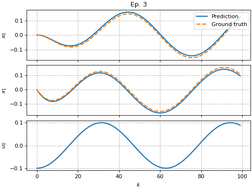
Simple Koopman pipeline
"""Example of how to use the Koopman pipeline."""
from matplotlib import pyplot as plt
from sklearn.preprocessing import MaxAbsScaler, StandardScaler
import pykoop
plt.rc('lines', linewidth=2)
plt.rc('axes', grid=True)
plt.rc('grid', linestyle='--')
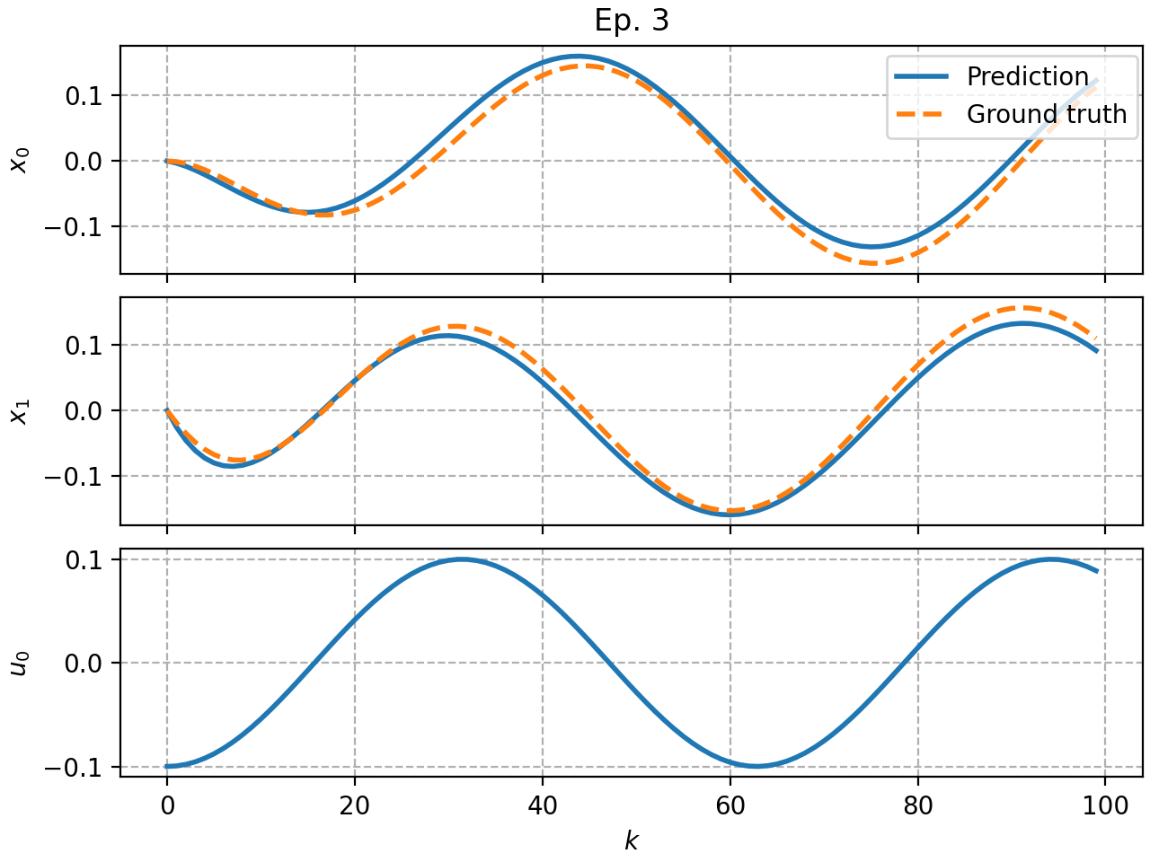
def example_pipeline_simple() -> None:
"""Demonstrate how to use the Koopman pipeline."""
# Get example mass-spring-damper data
eg = pykoop.example_data_msd()
# Create pipeline
kp = pykoop.KoopmanPipeline(
lifting_functions=[
('ma', pykoop.SkLearnLiftingFn(MaxAbsScaler())),
('pl', pykoop.PolynomialLiftingFn(order=2)),
('ss', pykoop.SkLearnLiftingFn(StandardScaler())),
],
regressor=pykoop.Edmd(alpha=1),
)
# Fit the pipeline
kp.fit(
eg['X_train'],
n_inputs=eg['n_inputs'],
episode_feature=eg['episode_feature'],
)
# Predict using the pipeline
X_pred = kp.predict_trajectory(eg['x0_valid'], eg['u_valid'])
# Score using the pipeline
score = kp.score(eg['X_valid'])
# Plot results
kp.plot_predicted_trajectory(eg['X_valid'], plot_input=True)
if __name__ == '__main__':
example_pipeline_simple()
plt.show()
(Source code, png, hires.png, pdf)

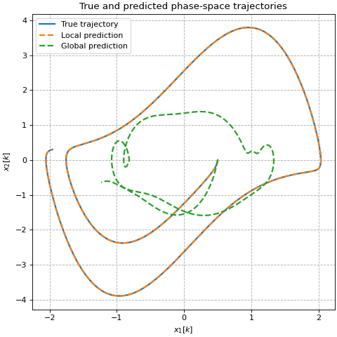
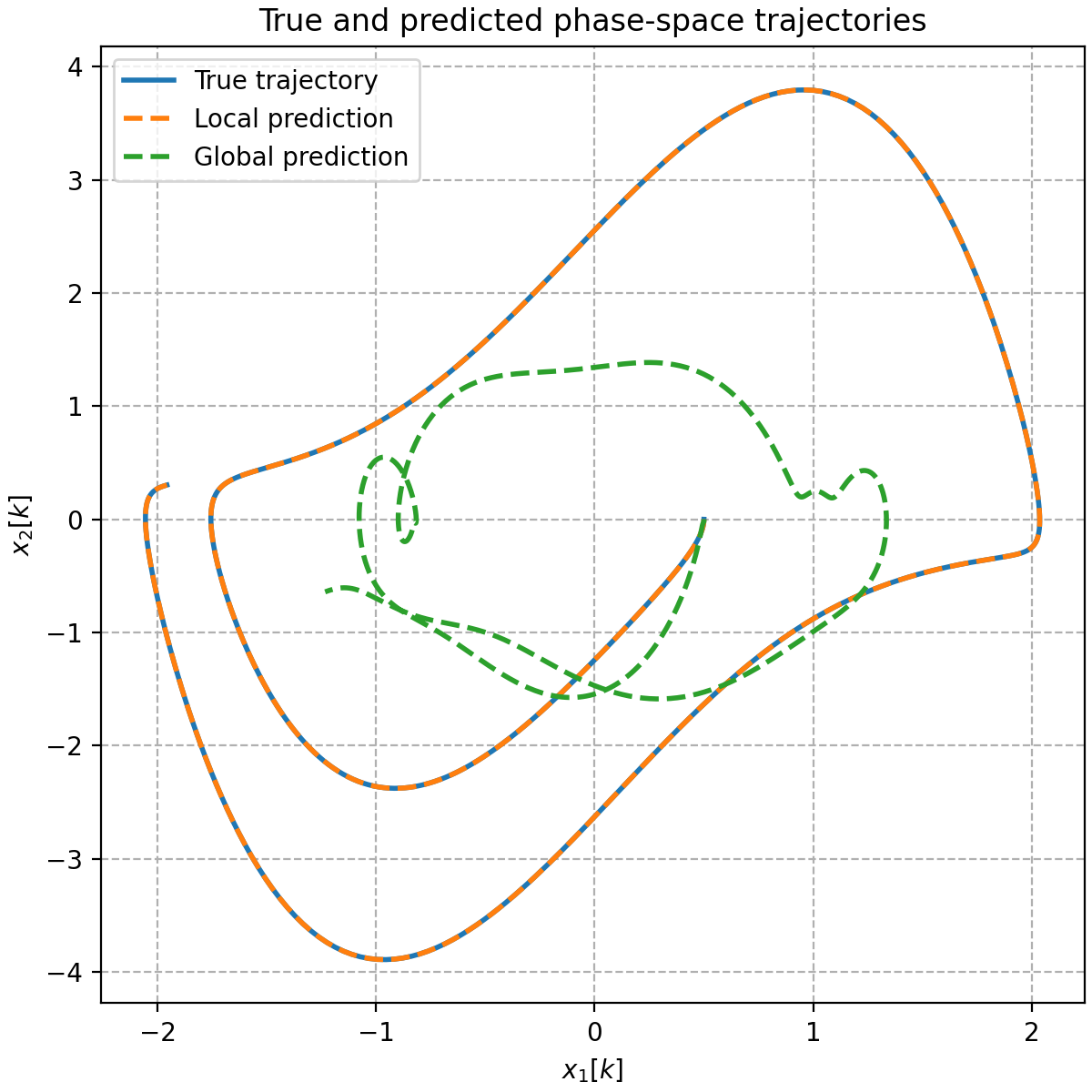
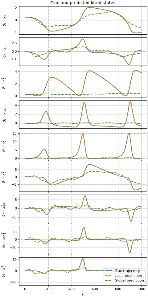
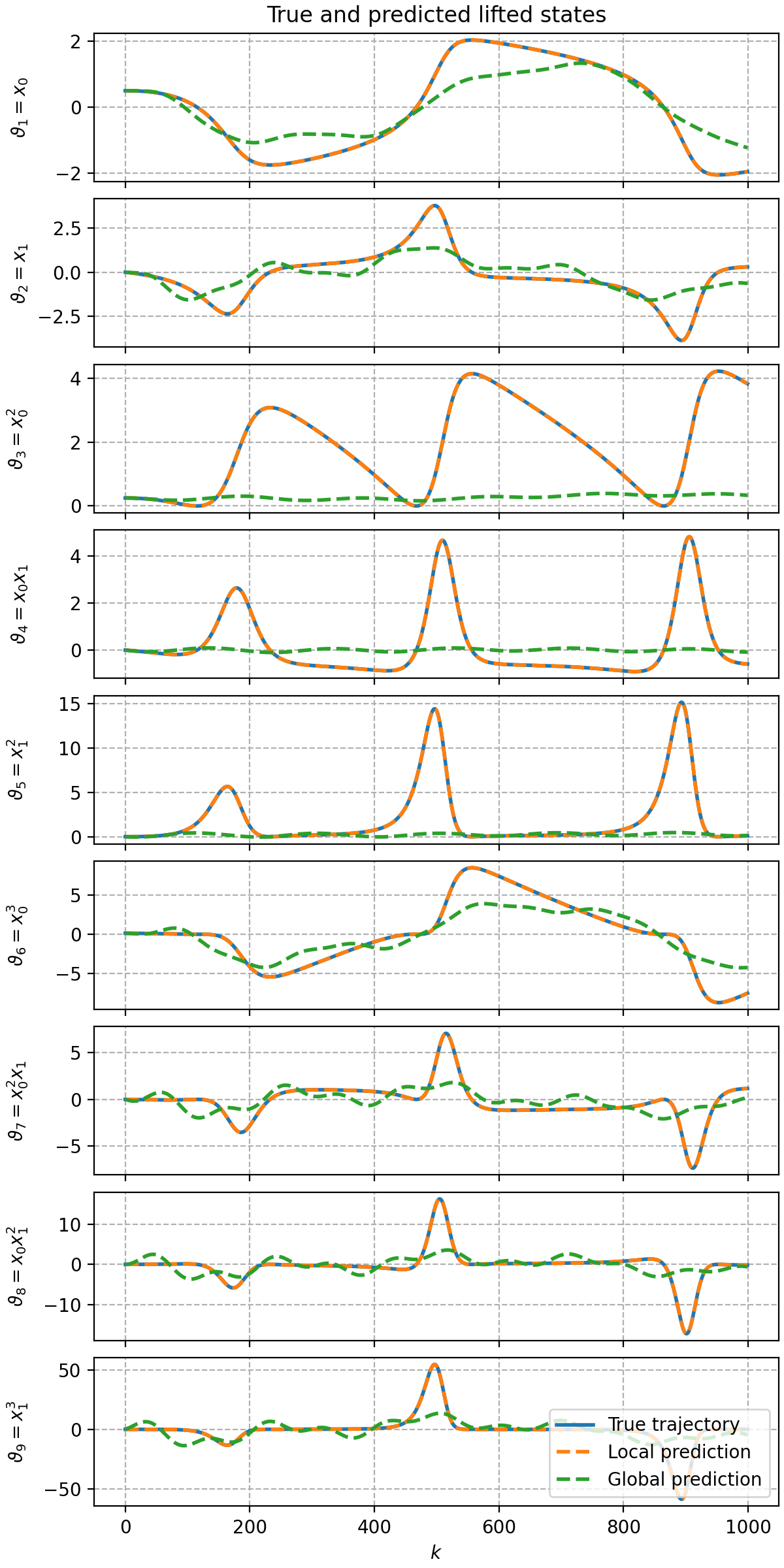
Van der Pol Oscillator
"""Example of how to use the Koopman pipeline."""

import numpy as np
from matplotlib import pyplot as plt

import pykoop

plt.rc('lines', linewidth=2)
plt.rc('axes', grid=True)
plt.rc('grid', linestyle='--')


def example_pipeline_vdp() -> None:
    """Demonstrate how to use the Koopman pipeline."""
    # Get example Van der Pol data
    eg = pykoop.example_data_vdp()

    # Create pipeline
    kp = pykoop.KoopmanPipeline(
        lifting_functions=[(
            'sp',
            pykoop.SplitPipeline(
                lifting_functions_state=[
                    ('pl', pykoop.PolynomialLiftingFn(order=3))
                ],
                lifting_functions_input=None,
            ),
        )],
        regressor=pykoop.Edmd(),
    )

    # Fit the pipeline
    kp.fit(
        eg['X_train'],
        n_inputs=eg['n_inputs'],
        episode_feature=eg['episode_feature'],
    )

    # Predict with re-lifting between timesteps (default)
    X_pred_local = kp.predict_trajectory(
        eg['x0_valid'],
        eg['u_valid'],
        relift_state=True,
    )

    # Predict without re-lifting between timesteps
    X_pred_global = kp.predict_trajectory(
        eg['x0_valid'],
        eg['u_valid'],
        relift_state=False,
    )

    # Plot trajectories in phase space
    fig, ax = plt.subplots(constrained_layout=True, figsize=(6, 6))
    ax.plot(
        eg['X_valid'][:, 1],
        eg['X_valid'][:, 2],
        label='True trajectory',
    )
    ax.plot(
        X_pred_local[:, 1],
        X_pred_local[:, 2],
        '--',
        label='Local prediction',
    )
    ax.plot(
        X_pred_global[:, 1],
        X_pred_global[:, 2],
        '--',
        label='Global prediction',
    )
    ax.set_xlabel('$x_1[k]$')
    ax.set_ylabel('$x_2[k]$')
    ax.legend()
    ax.set_title('True and predicted phase-space trajectories')

    # Lift validation set
    Psi_valid = kp.lift(eg['X_valid'])

    # Predict lifted state with re-lifting between timesteps (default)
    Psi_pred_local = kp.predict_trajectory(
        eg['x0_valid'],
        eg['u_valid'],
        relift_state=True,
        return_lifted=True,
        return_input=True,
    )

    # Predict lifted state without re-lifting between timesteps
    Psi_pred_global = kp.predict_trajectory(
        eg['x0_valid'],
        eg['u_valid'],
        relift_state=False,
        return_lifted=True,
        return_input=True,
    )

    # Get feature names
    names = kp.get_feature_names_out(format='latex')

    fig, ax = plt.subplots(
        kp.n_states_out_,
        1,
        constrained_layout=True,
        sharex=True,
        squeeze=False,
        figsize=(6, 12),
    )
    for i in range(ax.shape[0]):
        ax[i, 0].plot(
            Psi_valid[:, i + 1],
            label='True trajectory',
        )
        ax[i, 0].plot(
            Psi_pred_local[:, i + 1],
            '--',
            label='Local prediction',
        )
        ax[i, 0].plot(
            Psi_pred_global[:, i + 1],
            '--',
            label='Global prediction',
        )
        ax[i, 0].set_ylabel(rf'$\vartheta_{i + 1} = {names[i + 1]}$')

    ax[-1, 0].set_xlabel('$k$')
    ax[0, 0].set_title('True and predicted lifted states')
    ax[-1, -1].legend(loc='lower right')
    fig.align_ylabels()


if __name__ == '__main__':
    example_pipeline_vdp()
    plt.show()
Cross-validation with scikit-learn
To enable cross-validation, pykoop strives to be fully-compatible with
scikit-learn. All of its regressors and lifting functions pass
scikit-learn’s estimator checks, with minor exceptions made when
necessary.
Regressor parameters and lifting functions can easily be cross-validated using
scikit-learn:
"""Example of cross-validating lifting functions and regressor parameters."""

import numpy as np
import sklearn.model_selection
import sklearn.preprocessing
from matplotlib import pyplot as plt

import pykoop
import pykoop.dynamic_models

plt.rc('lines', linewidth=2)
plt.rc('axes', grid=True)
plt.rc('grid', linestyle='--')


def example_pipeline_cv() -> None:
    """Cross-validate regressor parameters."""
    # Get example mass-spring-damper data
    eg = pykoop.example_data_msd()

    # Create pipeline. Don't need to set lifting functions since they'll be set
    # during cross-validation.
    kp = pykoop.KoopmanPipeline(regressor=pykoop.Edmd())

    # Split data episode-by-episode
    episode_feature = eg['X_train'][:, 0]
    cv = sklearn.model_selection.GroupShuffleSplit(
        random_state=1234,
        n_splits=3,
    ).split(eg['X_train'], groups=episode_feature)

    # Define search parameters
    params = {
        # Lifting functions to try
        'lifting_functions': [
            [(
                'ss',
                pykoop.SkLearnLiftingFn(
                    sklearn.preprocessing.StandardScaler()),
            )],
            [
                (
                    'ma',
                    pykoop.SkLearnLiftingFn(
                        sklearn.preprocessing.MaxAbsScaler()),
                ),
                (
                    'pl',
                    pykoop.PolynomialLiftingFn(order=2),
                ),
                (
                    'ss',
                    pykoop.SkLearnLiftingFn(
                        sklearn.preprocessing.StandardScaler()),
                ),
            ],
        ],
        # Regressor parameters to try
        'regressor__alpha': [0, 0.1, 1, 10],
    }

    # Set up grid search
    gs = sklearn.model_selection.GridSearchCV(
        kp,
        params,
        cv=cv,
        # Score using short and long prediction time frames
        scoring={
            f'full_episode': pykoop.KoopmanPipeline.make_scorer(),
            f'ten_steps': pykoop.KoopmanPipeline.make_scorer(n_steps=10),
        },
        # Rank according to short time frame
        refit='ten_steps',
    )

    # Fit the pipeline
    gs.fit(
        eg['X_train'],
        n_inputs=eg['n_inputs'],
        episode_feature=eg['episode_feature'],
    )

    # Get results
    cv_results = gs.cv_results_
    best_estimator = gs.best_estimator_

    # Predict using the pipeline
    X_pred = best_estimator.predict_trajectory(eg['x0_valid'], eg['u_valid'])

    # Score using the pipeline
    score = best_estimator.score(eg['X_valid'])

    # Plot results
    best_estimator.plot_predicted_trajectory(eg['X_valid'], plot_input=True)


if __name__ == '__main__':
    example_pipeline_cv()
    plt.show()
(Source code, png, hires.png, pdf)

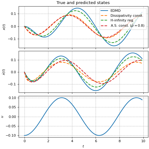
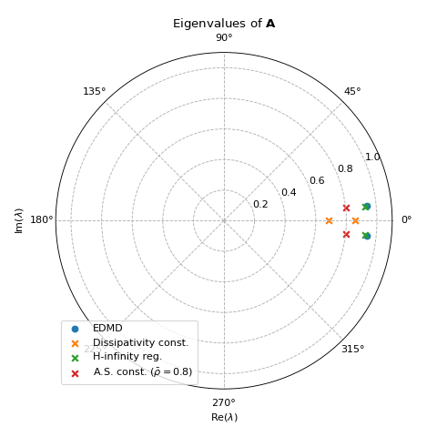
Asymptotic stability constraint
In this example, three experimental EDMD-based regressors are compared to EDMD. Specifically, EDMD is compared to the asymptotic stability constraint and the H-infinity norm regularizer from [DF22] and [DF21], and the dissipativity constraint from [HIS19].
"""Example comparing eigenvalues of different versions of EDMD."""

import numpy as np
from matplotlib import pyplot as plt
from scipy import integrate, linalg

import pykoop
import pykoop.lmi_regressors

plt.rc('lines', linewidth=2)
plt.rc('axes', grid=True)
plt.rc('grid', linestyle='--')


def example_eigenvalue_comparison() -> None:
    """Compare eigenvalues of different versions of EDMD."""
    # Get example data
    eg = pykoop.example_data_msd()
    # Set solver (you can switch to ``'mosek'`` if you have a license).
    solver = 'cvxopt'

    # Regressor with no constraint
    reg_no_const = pykoop.KoopmanPipeline(regressor=pykoop.Edmd())
    reg_no_const.fit(
        eg['X_train'],
        n_inputs=eg['n_inputs'],
        episode_feature=eg['episode_feature'],
    )
    U_no_const = reg_no_const.regressor_.coef_.T

    # Regressor H-infinity norm constraint of 1.5
    gamma = 1.5
    Xi = np.block([
        [1 / gamma * np.eye(2), np.zeros((2, 1))],
        [np.zeros((1, 2)), -gamma * np.eye(1)],
    ])  # yapf: disable
    reg_diss_const = pykoop.KoopmanPipeline(
        regressor=pykoop.lmi_regressors.LmiEdmdDissipativityConstr(
            supply_rate=Xi,
            solver_params={'solver': solver},
        ))
    reg_diss_const.fit(
        eg['X_train'],
        n_inputs=eg['n_inputs'],
        episode_feature=eg['episode_feature'],
    )
    U_diss_const = reg_diss_const.regressor_.coef_.T

    # Regressor with H-infinity regularization
    reg_hinf_reg = pykoop.KoopmanPipeline(
        regressor=pykoop.lmi_regressors.LmiEdmdHinfReg(
            alpha=1e-2,
            solver_params={'solver': solver},
        ))
    reg_hinf_reg.fit(
        eg['X_train'],
        n_inputs=eg['n_inputs'],
        episode_feature=eg['episode_feature'],
    )
    U_hinf_reg = reg_hinf_reg.regressor_.coef_.T

    # Regressor with spectral radius constraint
    reg_sr_const = pykoop.KoopmanPipeline(
        regressor=pykoop.lmi_regressors.LmiEdmdSpectralRadiusConstr(
            spectral_radius=0.8,
            solver_params={'solver': solver},
        ))
    reg_sr_const.fit(
        eg['X_train'],
        n_inputs=eg['n_inputs'],
        episode_feature=eg['episode_feature'],
    )
    U_sr_const = reg_sr_const.regressor_.coef_.T

    # Predict using the pipeline
    X_pred_no_const = reg_no_const.predict_trajectory(
        eg['x0_valid'],
        eg['u_valid'],
    )
    X_pred_diss_const = reg_diss_const.predict_trajectory(
        eg['x0_valid'],
        eg['u_valid'],
    )
    X_pred_hinf_reg = reg_hinf_reg.predict_trajectory(
        eg['x0_valid'],
        eg['u_valid'],
    )
    X_pred_sr_const = reg_sr_const.predict_trajectory(
        eg['x0_valid'],
        eg['u_valid'],
    )

    # Plot results
    fig, ax = plt.subplots(
        reg_no_const.n_states_in_ + reg_no_const.n_inputs_in_,
        1,
        constrained_layout=True,
        sharex=True,
        figsize=(6, 6),
    )
    # Plot input
    ax[2].plot(eg['t'], eg['X_valid'][:, 3])
    # Plot predicted trajectory
    ax[0].plot(eg['t'], X_pred_no_const[:, 1], label='EDMD')
    ax[1].plot(
        eg['t'],
        X_pred_no_const[:, 2],
    )
    ax[0].plot(
        eg['t'],
        X_pred_diss_const[:, 1],
        '--',
        label='Dissipativity const.',
    )
    ax[1].plot(eg['t'], X_pred_diss_const[:, 2], '--')
    ax[0].plot(
        eg['t'],
        X_pred_hinf_reg[:, 1],
        '--',
        label='H-infinity reg.',
    )
    ax[1].plot(eg['t'], X_pred_hinf_reg[:, 2], '--')
    ax[0].plot(
        eg['t'],
        X_pred_sr_const[:, 1],
        '--',
        label=r'A.S. const. ($\bar{\rho}=0.8$)',
    )
    ax[1].plot(
        eg['t'],
        X_pred_sr_const[:, 2],
        '--',
    )
    # Add labels
    ax[-1].set_xlabel('$t$')
    ax[0].set_ylabel('$x(t)$')
    ax[1].set_ylabel(r'$\dot{x}(t)$')
    ax[2].set_ylabel('$u$')
    ax[0].set_title(f'True and predicted states')
    ax[0].legend(loc='upper right')

    # Plot results
    fig = plt.figure(figsize=(6, 6))
    ax = plt.subplot(projection='polar')
    ax.set_xlabel(r'$\mathrm{Re}(\lambda)$')
    ax.set_ylabel(r'$\mathrm{Im}(\lambda)$', labelpad=30)
    plt_eig(U_no_const[:2, :2], ax, 'EDMD', marker='o')
    plt_eig(U_diss_const[:2, :2], ax, r'Dissipativity const.')
    plt_eig(U_hinf_reg[:2, :2], ax, r'H-infinity reg.')
    plt_eig(
        U_sr_const[:2, :2],
        ax,
        r'A.S. const. ($\bar{\rho}=0.8$)',
    )
    ax.set_rmax(1.1)
    ax.legend(loc='lower left')
    ax.set_title(r'Eigenvalues of $\bf{A}$')


def plt_eig(A: np.ndarray,
            ax: plt.Axes,
            label: str = '',
            marker: str = 'x') -> None:
    """Eigenvalue plotting helper function."""
    eigv = linalg.eig(A)[0]
    ax.scatter(np.angle(eigv), np.absolute(eigv), marker=marker, label=label)


if __name__ == '__main__':
    example_eigenvalue_comparison()
    plt.show()


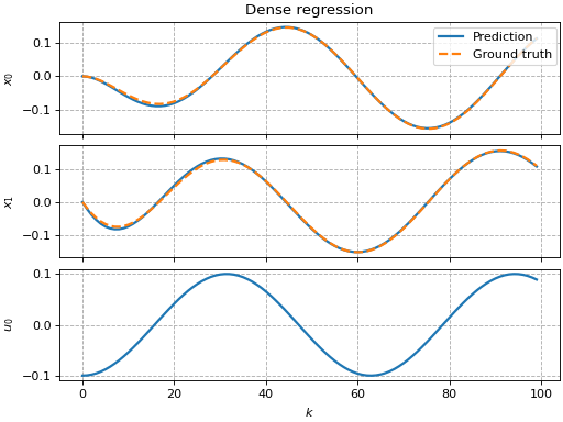
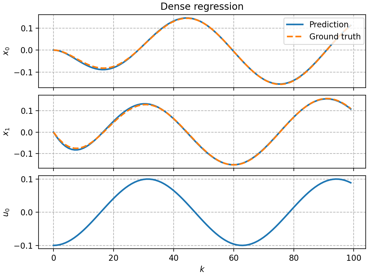
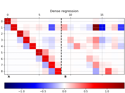
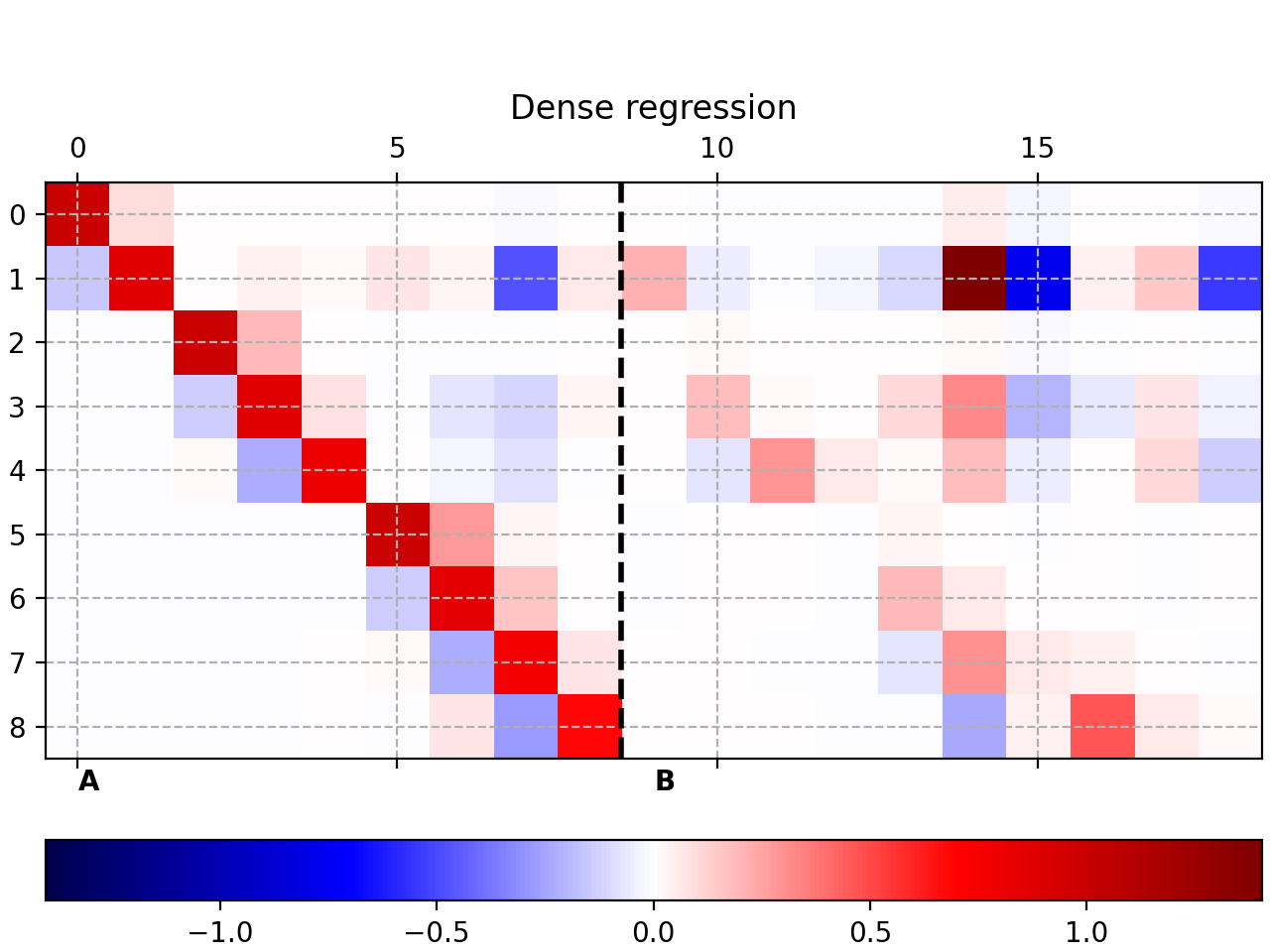
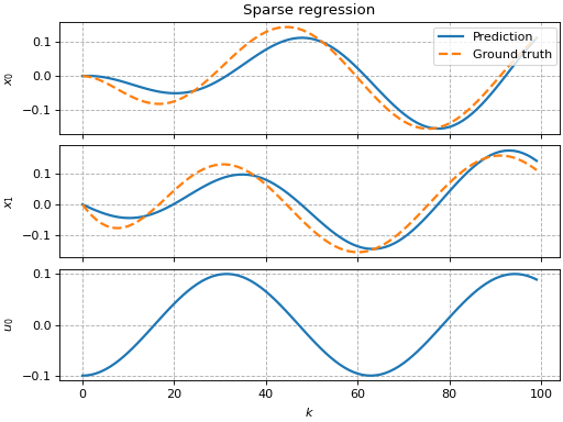
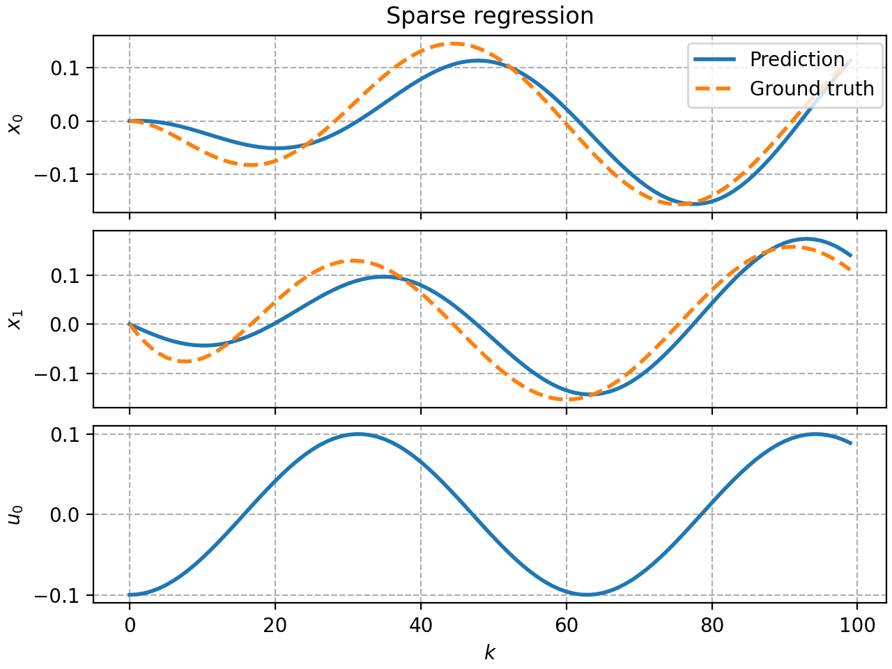
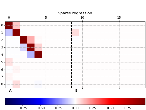
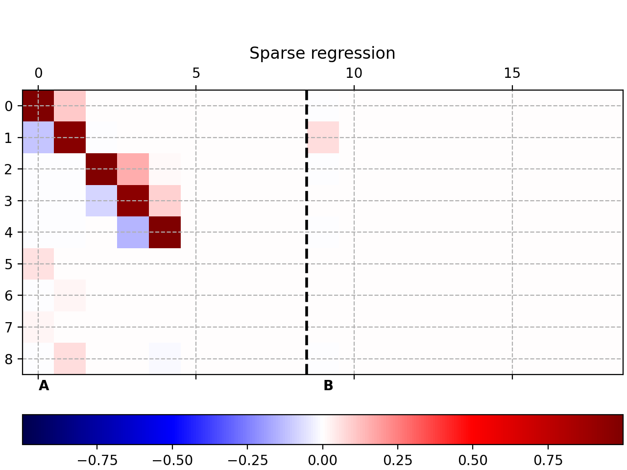
Sparse regression
This example shows how to use pykoop.EdmdMeta to implement sparse
regression with sklearn.linear_model.Lasso. The lasso promotes empty
columns in the Koopman matrix, which means the corresponding lifting functions
can be removed from the model.
"""Example of sparse regression with :class:`EdmdMeta`."""

from matplotlib import pyplot as plt
from sklearn.linear_model import Lasso

import pykoop

plt.rc('lines', linewidth=2)
plt.rc('axes', grid=True)
plt.rc('grid', linestyle='--')


def example_sparse_regression() -> None:
    """Demonstrate sparse regression with :class:`EdmdMeta`."""
    # Get example mass-spring-damper data
    eg = pykoop.example_data_msd()

    # Choose lifting functions
    poly3 = [('pl', pykoop.PolynomialLiftingFn(order=3))]

    # Create dense pipeline
    kp_dense = pykoop.KoopmanPipeline(
        lifting_functions=poly3,
        regressor=pykoop.Edmd(alpha=1e-9),
    )
    # Create sparse pipeline
    kp_sparse = pykoop.KoopmanPipeline(
        lifting_functions=poly3,
        # Also try out :class:`sklearn.linear_model.OrthogonalMatchingPursuit`!
        regressor=pykoop.EdmdMeta(regressor=Lasso(alpha=1e-9)),
    )

    # Fit the pipelines
    kp_dense.fit(
        eg['X_train'],
        n_inputs=eg['n_inputs'],
        episode_feature=eg['episode_feature'],
    )
    kp_sparse.fit(
        eg['X_train'],
        n_inputs=eg['n_inputs'],
        episode_feature=eg['episode_feature'],
    )

    # Plot dense prediction and Koopman matrix
    fig, ax = kp_dense.plot_predicted_trajectory(
        eg['X_valid'],
        plot_input=True,
    )
    ax[0, 0].set_title('Dense regression')
    fig, ax = kp_dense.plot_koopman_matrix()
    ax.set_title('Dense regression')

    # Plot sparse prediction and Koopman matrix
    fig, ax = kp_sparse.plot_predicted_trajectory(
        eg['X_valid'],
        plot_input=True,
    )
    ax[0, 0].set_title('Sparse regression')
    fig, ax = kp_sparse.plot_koopman_matrix()
    ax.set_title('Sparse regression')


if __name__ == '__main__':
    example_sparse_regression()
    plt.show()

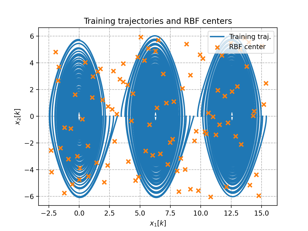
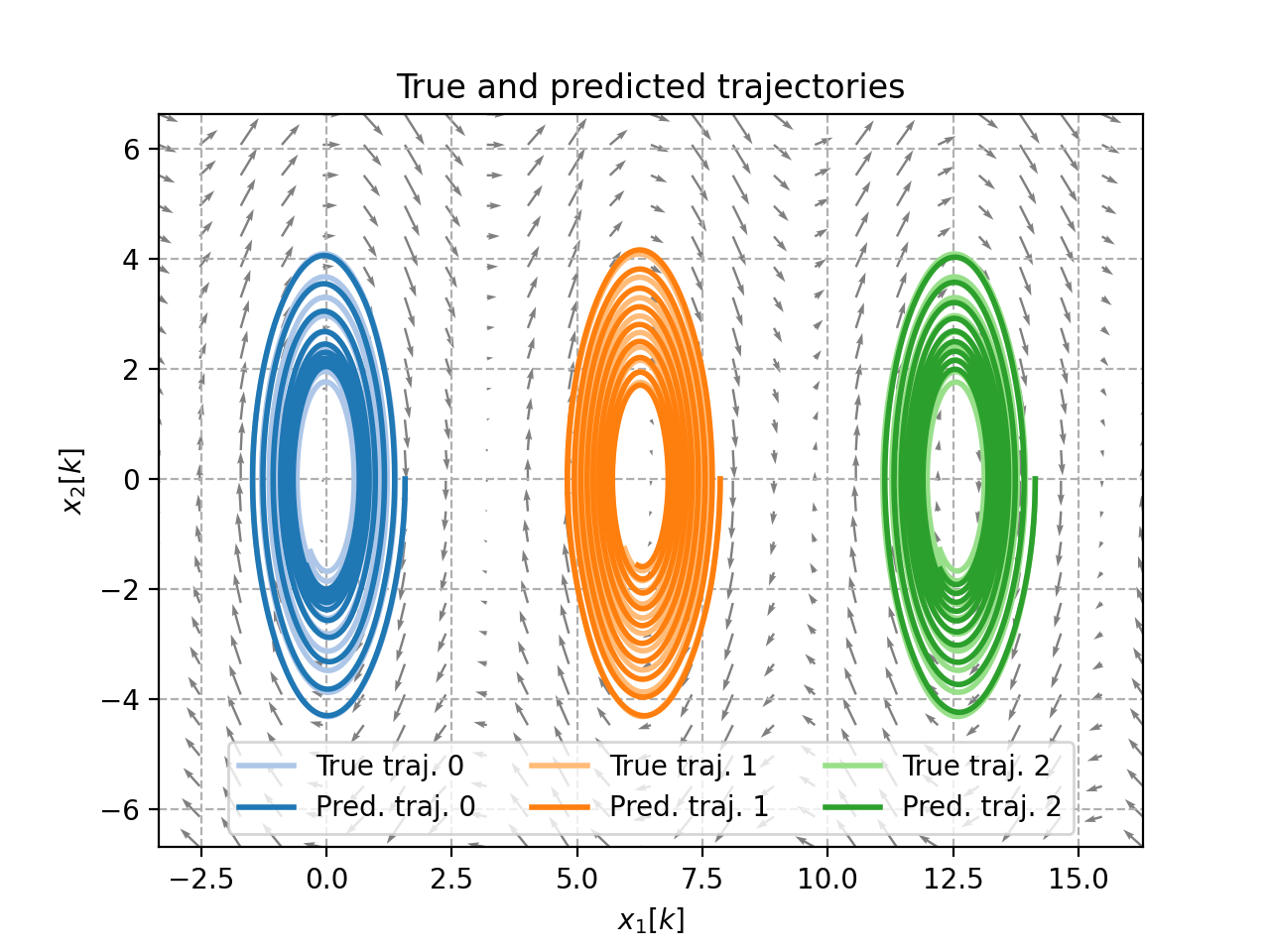
Radial basis functions on a pendulum
This example shows how thin-plate radial basis functions can be used as lifting functions to identify pendulum dynamics (where all trajectories have zero initial velocity). Latin hypercube sampling is used to generate 100 centers.
"""Example of radial basis functions on a pendulum."""
import numpy as np
import scipy.stats
from matplotlib import pyplot as plt

import pykoop

plt.rc('lines', linewidth=2)
plt.rc('axes', grid=True)
plt.rc('grid', linestyle='--')


def example_radial_basis_functions() -> None:
    """Demonstrate radial basis functions on a pendulum."""
    # Get example pendulum data
    eg = pykoop.example_data_pendulum()

    # Create pipeline
    kp = pykoop.KoopmanPipeline(
        lifting_functions=[(
            'rbf',
            pykoop.RbfLiftingFn(
                rbf='thin_plate',
                centers=pykoop.QmcCenters(
                    n_centers=100,
                    qmc=scipy.stats.qmc.LatinHypercube,
                    random_state=666,
                ),
            ),
        )],
        regressor=pykoop.Edmd(),
    )

    # Fit the pipeline
    kp.fit(
        eg['X_train'],
        n_inputs=eg['n_inputs'],
        episode_feature=eg['episode_feature'],
    )

    # Get training and validation episodes
    ep_train = np.unique(eg['X_train'][:, 0])
    ep_valid = np.unique(eg['X_valid'][:, 0])

    # Plot training trajectories
    fig, ax = plt.subplots()
    for ep in ep_train:
        idx = eg['X_train'][:, 0] == ep
        cax_line = ax.plot(
            eg['X_train'][idx, 1],
            eg['X_train'][idx, 2],
            color='C0',
        )
    # Plot centers
    c = kp.lifting_functions_[0][1].centers_.centers_
    for i in range(c.shape[0]):
        cax_scatter = ax.scatter(
            c[i, 0],
            c[i, 1],
            color='C1',
            marker='x',
            zorder=2,
        )
    # Set legend
    ax.legend(
        [cax_line[0], cax_scatter],
        [
            'Training traj.',
            'RBF center',
        ],
        loc='upper right',
    )
    # Set labels
    ax.set_title('Training trajectories and RBF centers')
    ax.set_xlabel('$x_1[k]$')
    ax.set_ylabel('$x_2[k]$')
    # Save axis limits for next figure
    xlim = ax.get_xlim()
    ylim = ax.get_ylim()

    # Predict new trajectories
    X_pred = kp.predict_trajectory(
        eg['x0_valid'],
        eg['u_valid'],
    )

    # Plot validation trajectories
    fig, ax = plt.subplots()
    tab20 = plt.cm.tab20(np.arange(0, 1, 0.05))
    color = [
        (tab20[1], tab20[0]),
        (tab20[3], tab20[2]),
        (tab20[5], tab20[4]),
    ]
    for (i, ep) in enumerate(ep_valid):
        idx = eg['X_valid'][:, 0] == ep
        cax_valid = ax.plot(
            eg['X_valid'][idx, 1],
            eg['X_valid'][idx, 2],
            color=color[i][0],
            label=f'True traj. {i}',
        )
        cax_pred = ax.plot(
            X_pred[idx, 1],
            X_pred[idx, 2],
            label=f'Pred. traj. {i}',
        )
    # Set axis limits
    ax.set_xlim(*xlim)
    ax.set_ylim(*ylim)
    # Plot true vector field
    pend = eg['dynamic_model']
    xx, yy = np.meshgrid(np.linspace(*xlim, 25), np.linspace(*ylim, 25))
    x = np.vstack((xx.ravel(), yy.ravel()))
    x_dot = np.array([pend.f(0, x[:, k], 0) for k in range(x.shape[1])]).T
    ax.quiver(x[0, :], x[1, :], x_dot[0, :], x_dot[1, :], color='grey')
    # Set legend
    ax.legend(loc='lower center', ncol=3)
    # Set labels
    ax.set_title('True and predicted trajectories')
    ax.set_xlabel('$x_1[k]$')
    ax.set_ylabel('$x_2[k]$')


if __name__ == '__main__':
    example_radial_basis_functions()
    plt.show()


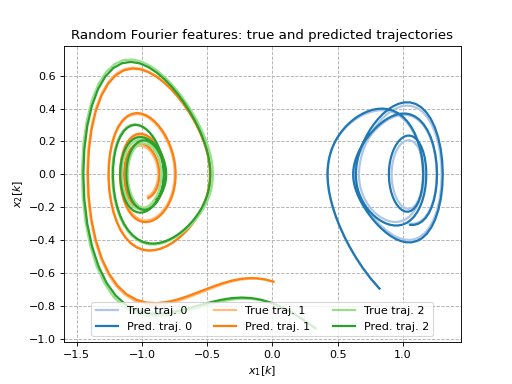
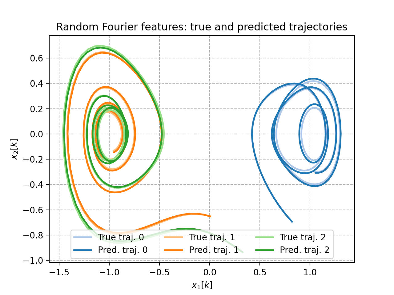
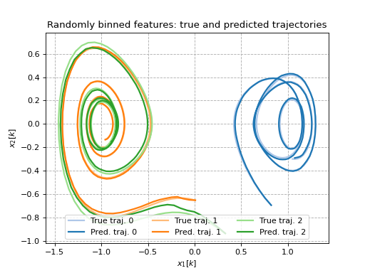
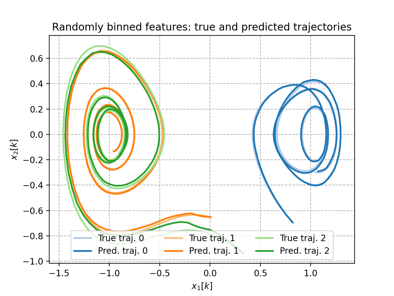
Random Fourier features on a Duffing oscillator
This example shows how random Fourier features (and randomly binned features) can be used as lifting functions to identify Duffing oscillator dynamics. For more details on how these features are generated, see [RR07].
"""Example of random Fourier features on a Duffing oscillator."""
import numpy as np
import scipy.stats
from matplotlib import pyplot as plt

import pykoop

plt.rc('lines', linewidth=2)
plt.rc('axes', grid=True)
plt.rc('grid', linestyle='--')


def example_random_fourier_features() -> None:
    """Demonstrate random Fourier featuers on a Duffing oscillator."""
    # Get example Duffing oscillator data
    eg = pykoop.example_data_duffing()

    # Create RFF pipeline
    kp_rff = pykoop.KoopmanPipeline(
        lifting_functions=[(
            'rff',
            pykoop.KernelApproxLiftingFn(
                kernel_approx=pykoop.RandomFourierKernelApprox(
                    n_components=100,
                    random_state=1234,
                )),
        )],
        regressor=pykoop.Edmd(),
    )

    # Create random binning pipeline for comparison
    kp_bin = pykoop.KoopmanPipeline(
        lifting_functions=[(
            'bin',
            pykoop.KernelApproxLiftingFn(
                kernel_approx=pykoop.RandomBinningKernelApprox(
                    n_components=10,
                    random_state=1234,
                )),
        )],
        regressor=pykoop.Edmd(),
    )

    for label, kp in [
        ('Random Fourier features', kp_rff),
        ('Randomly binned features', kp_bin),
    ]:
        # Fit the pipeline
        kp.fit(
            eg['X_train'],
            n_inputs=eg['n_inputs'],
            episode_feature=eg['episode_feature'],
        )

        # Get training and validation episodes
        ep_train = np.unique(eg['X_train'][:, 0])
        ep_valid = np.unique(eg['X_valid'][:, 0])

        # Predict new trajectories
        X_pred = kp.predict_trajectory(
            eg['x0_valid'],
            eg['u_valid'],
        )

        # Plot validation trajectories
        fig, ax = plt.subplots()
        tab20 = plt.cm.tab20(np.arange(0, 1, 0.05))
        color = [
            (tab20[1], tab20[0]),
            (tab20[3], tab20[2]),
            (tab20[5], tab20[4]),
        ]
        for (i, ep) in enumerate(ep_valid):
            idx = eg['X_valid'][:, 0] == ep
            cax_valid = ax.plot(
                eg['X_valid'][idx, 1],
                eg['X_valid'][idx, 2],
                color=color[i][0],
                label=f'True traj. {i}',
            )
            cax_pred = ax.plot(
                X_pred[idx, 1],
                X_pred[idx, 2],
                label=f'Pred. traj. {i}',
            )
        # Set legend
        ax.legend(loc='lower center', ncol=3)
        # Set labels
        ax.set_title(f'{label}: true and predicted trajectories')
        ax.set_xlabel('$x_1[k]$')
        ax.set_ylabel('$x_2[k]$')


if __name__ == '__main__':
    example_random_fourier_features()
    plt.show()

